Stationary Tests (R)
Tests of stationarity
This is the second post on ARIMA time series forecasting method. In the first post, we discussed stationarity, random walk and other concepts. In this blog, we are going to discuss various ways one can test for stationarity.
Two types of tests are introduced in this blog
1. Unit root tests
2. Independence tests
Data
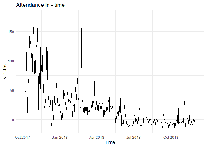
For the following blog, we will use a sample from attendance data set described in EDA blogs.
From the time series and ACF plots, one can observe non-stationarity and decreasing trend.

Unit root tests
As discussed in the previous blog, unit root stochastic process is another name for Random walk process. A random walk process can be written as $$ Y_t=\rho \times Y_{t−1} + \epsilon_t $$ Where \(\rho = 1\). If \(|\rho|<1\) then the process represents Markov first order auto regressive model which is stationary. Only for \(\rho=1\) we get non-stationary.
The above equation can be alternatively written as $$ Y_t - Y_{t-1} = \Delta Y_t = \delta \times Y_{t-1} + \epsilon_t $$ Where \(\delta = \rho -1\). For non-stationarity, the condition now becomes \(\delta = 0\) the alternative hypothesis being \(\delta < 0\). The null and alternate hypothesis are:
$$ H_0: \delta = 0 $$ $$ H_1 : \delta < 0 $$ Under this null hypothesis, \(Y_{t-1}\) does not follow a normal distribution(or t-distribution).
Dickey and Fuller have shown that for the above null and alternate hypothesis, the estimated test statistic follows the \(\tau\) statistic. If the hypothesis that \(\delta=0\) is rejected, that is if the series is stationary, then we can use the t-test for further analysis.
Dickey Fuller tests
The Dickey fuller tests contains two steps.
1. Test if the series is stationary
2. If the series is not stationary, test what kind of non-stationarity is present
As non-stationarity can exist in three ways, the dickey fuller test is estimated in three different forms
\(Y_t\) is a random walk : \(\Delta Y_t = \delta Y_{t-1} + \epsilon_t\)
\(Y_t\) is a random walk with drift : \(\Delta Y_t = \beta_1 + \delta Y_{t-1} + \epsilon_t\)
\(Y_t\) is a random walk with drift around a deterministic trend : \(\Delta Y_t = \beta_1 + \beta_2 t +\delta Y_{t-1} + \epsilon_t\)
In each case, the null hypothesis is that \(\delta = 0\), i.e., there is a unit root—the time series is non-stationary. The alternative hypothesis is that \(\delta < 0\) that is, the time series is stationary.
If the null hypothesis is rejected, it means the following in the three scenarios:
1. \(Y_t\) is a stationary time series with zero mean in the case of random walk
2. \(Y_t\) is stationary with a non-zero mean in the case of random walk with drift
3. \(Y_t\) is stationary around a deterministic trend in case of random walk with drift around a deterministic trend
The actual estimation procedure is as follows:
1. Perform the tests from backwards, i.e., estimate deterministic trend first, then random walk with drift and then random walk. This is to ensure we are not committing specification error
2. For the three tests, estimate the \(\tau\) statistic and compare with the (MacKinnon) critical tau values, If the computed absolute value of the tau statistic (\(|\tau|\)) exceeds the critical tau values, we reject the Null hypothesis in which case the time series is stationary
3. If any of the (\(\tau\)) values are less than the critical tau value, then we retain the Null hypothesis in which case the time series is non-stationary. The critical \(\tau\) values can vary between the three tests
For the attendance data, the Dickey fuller tests give the following results:
## ========================================================================
## At the 5pct level:
## The test is for type random walk
## delta=0: The null hypothesis is not rejected, the series is not stationary
## ========================================================================
## ========================================================================
## At the 5pct level:
## The test is for type random walk with drift
## delta=0: The first null hypothesis is not rejected, the series is not stationary
## delta=0 and beta1=0: The second null hypothesis is rejected, the series is not stationary
##       and there is drift.
## ========================================================================
## ========================================================================
## At the 5pct level:
## The test is for type random walk with drift and deterministic trend
## delta=0: The first null hypothesis is not rejected, the series is not stationary
## delta=0 and beta2=0: The second null hypothesis is rejected, the series is not stationary
##       and there is trend
## delta=0 and beta1=0 and beta2=0: The third null hypothesis is rejected, the series is not stationary
##       there is trend, and there may or may not be drift
## Warning in interp_urdf(ur.df(time.series, type = "trend")): Presence of drift is inconclusive.
## ========================================================================
The above result should be interpreted as follows (read backwards):
3. There might be a deterministic trend in the series there may or may not be a drift coefficient
2. The series is non-stationary and there is drift coefficient
1. The series is non-stationary
Therefore, the series is not stationary.
Augmented Dickey−Fuller Test
In conducting the DF test, it was assumed that the error term was uncorrelated. But in case the \(\epsilon_t\) are correlated, Dickey and Fuller have developed a test, known as the augmented Dickey–Fuller (ADF) test. This test is conducted by “augmenting” the three equations by adding the lagged values of the dependent variable. The null hypothesis and alternative hypothesis are given by
\(H_0\): \(\gamma\) = 0 (the time series is non-stationary)
\(H_1\): \(\gamma\) < 0 (the time series is stationary)
Where $$ \Delta y_t = \alpha + \beta t + \gamma y_{t-1} + \delta_1 \Delta y_{t-1} + \delta_2 \Delta y_{t-2} + \dots $$
Ljung–Box independence test
Ljung−Box is a test of lack of fit of the forecasting model and checks whether the auto-correlations for the errors are different from zero. The null and alternative hypotheses are given by
\(H_0\): The model does not show lack of fit
\(H_1\): The model exhibits lack of fit
The Ljung−Box statistic (Q-Statistic) is given by $$ Q(m) = n(n+2) \sum_{k=1}{m}\frac{\rho_k2}{n-k}$$ where n is the number of observations in the time series, k is the number of lag, \(r_k\) is the auto-correlation of lag k, and m is the total number of lags. Q-statistic is an approximate chi-square distribution with m – p – q degrees of freedom where p and q are the AR and MA lags.
##
##  Box-Ljung test
##
## data:  time.series
## X-squared = 1070.9, df = 10, p-value < 2.2e-16
References
- Basic Ecnometrics - Damodar N Gujarati
- SAS for Forecasting Time Series, Third Edition - Dickey
- Customer Analytics at Flipkart.Com - Naveen Bhansali (case study in Harvard business review)
- This discussion on stack overflow