Arima forecasting
Air pollution is a major issue in Hyderabad where I live. I am using the data taken from aqicn.org on the PM25 pollutant near my house in Hyderabad, India. I am using this data to build a model that will predict the PM25 air quality near my home. The training data can be found at aqicn's API
This model is deployed on a flask application at harshaash.pythonanywhere.com as a Rest API and you can find the past and current results at hydpm25.aharsha.com/. The details on how to deploy the models can be found in the blog ML Deployment in Flask.
To find the theory of ARIMA in detail, read the blogs on Stationarity, Tests for stationarity and ARIMA concept.
import warnings
warnings.filterwarnings('ignore', category=FutureWarning)

%matplotlib inline

import pandas as pd
import matplotlib.pyplot as plt
import seaborn as sns
data = pd.read_csv('hyderabad-us consulate-air-quality.csv', parse_dates=['date'])
Visualising time series
Historic data is present in the form of daily average since 2014 December.
data = data.sort_values('date')
data.columns = ['date', 'pm25']
data
| date | pm25 | |
|---|---|---|
| 2295 | 2014-12-10 | 172 |
| 2296 | 2014-12-11 | 166 |
| 2297 | 2014-12-12 | 159 |
| 2298 | 2014-12-13 | 164 |
| 2299 | 2014-12-14 | 166 |
| ... | ... | ... |
| 0 | 2021-11-01 | 155 |
| 1 | 2021-11-02 | 115 |
| 2 | 2021-11-03 | 67 |
| 3 | 2021-11-04 | 112 |
| 4 | 2021-11-05 | 115 |
2314 rows × 2 columns
plt.figure(figsize=(20,10))
plt.plot(data.date, data.pm25, color='tab:red')
plt.gca().set(title='Pollution at Hyderabad', xlabel='Date', ylabel='PM25')
plt.show()
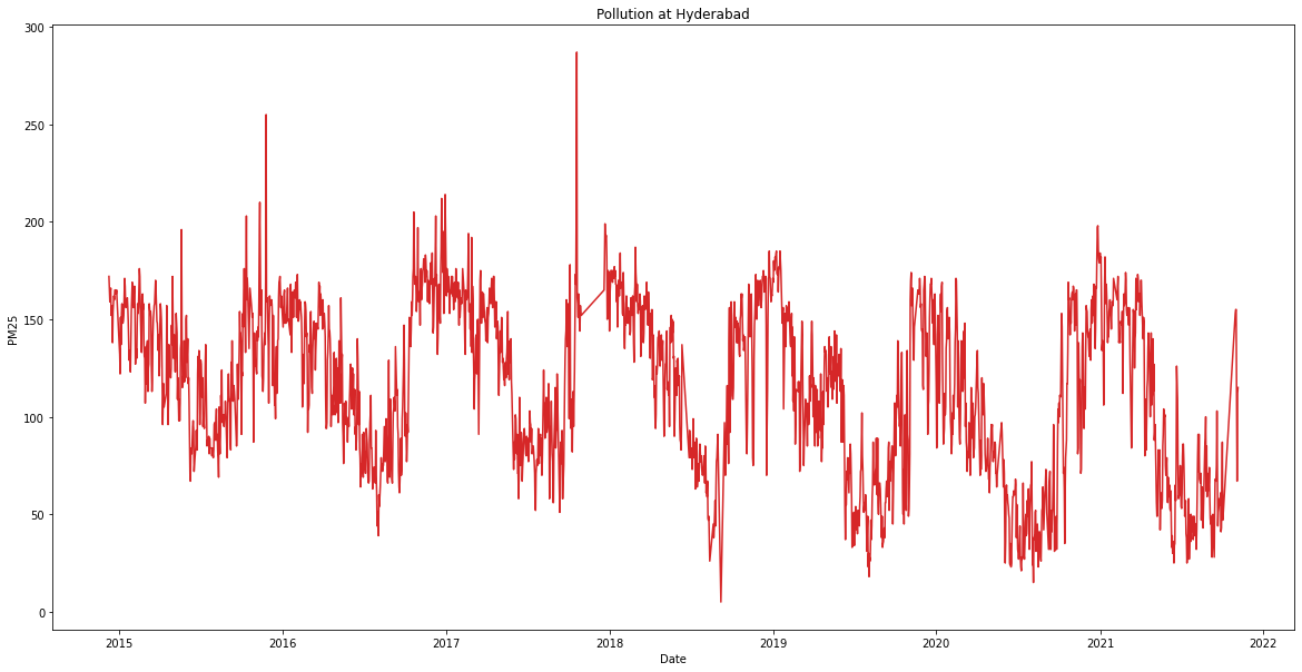
From this plot, we can see that pollution is higher during winter months while its lower during summer months. This effect is observed every year indicating a seasonal pattern in the data. There seems to be no increasing or decreasing trend in the data. This can be better visualised by decomposing the data into three components:
1. Seasonal component: The component that varies with season
2. Trend: Increasing or decreasing pattern
3. Random component: Remaining component that has no pattern
from statsmodels.tsa.seasonal import seasonal_decompose
result = seasonal_decompose(data.pm25, model='additive', period = 365)
fs, axs = plt.subplots(3, figsize=(20,10))
plt.suptitle('Pollution (PM25) at Hyderabad', fontsize = 20, y = 0.95)

axs[0].plot(data.date, result.trend)
axs[1].plot(data.date, result.seasonal)
axs[2].plot(data.date, result.resid)

axs[0].set_ylabel('Trend', fontsize=15)
axs[1].set_ylabel('Seasonality', fontsize=15)
axs[2].set_ylabel('Random component', fontsize=15)

plt.show()
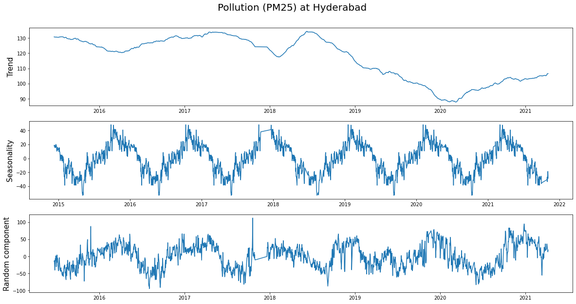
Looking at the trend, we can see how the pollution decreased during 2020 (probably due to covid) and is slowly rising as the country is getting back to its feet.
data['year'] = data.date.dt.year
data['day'] = data.date.dt.dayofyear
plt.figure(figsize=(16,12), dpi= 80)
for i, y in enumerate(data.year.unique()):
plt.plot('day', 'pm25', data=data.loc[data.year==y, :], label = y)
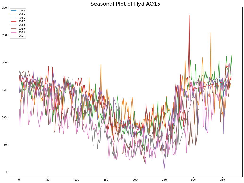
plt.title("Seasonal Plot of Hyd AQ15", fontsize=20)
plt.legend(loc="upper left")
Dickey Fuller unit root test
To find out if a time series is stationary, we can use the Dickey Fuller test. As discussed in the previous blog[], unit root stochastic process is another name for Random walk process. A random walk process can be written as
$$ Y_t=\rho \times Y_{t−1} + \epsilon_t $$
Where \(\rho = 1\). If \(|\rho|<1\) then the process represents Markov first order auto regressive model which is stationary. Only for \(\rho=1\) we get non-stationary.
The above equation can be alternatively written as $$ Y_t - Y_{t-1} = \Delta Y_t = \delta \times Y_{t-1} + \epsilon_t $$ Where \(\delta = \rho -1\). For non-stationarity, the condition now becomes \(\delta = 0\) the alternative hypothesis being \(\delta < 0\). The null and alternate hypothesis are:
\(H_0: \delta = 0\) (Time series is non-stationary)
\(H_1 : \delta < 0\) (Time series is stationary)
Under this null hypothesis, \(Y_{t-1}\) does not follow a normal distribution(or t-distribution).
Dickey and Fuller have shown that for the above null and alternate hypothesis, the estimated test statistic follows the \(\tau\) statistic. If the hypothesis that \(\delta=0\) is rejected, that is if the series is stationary, then we can use the t-test for further analysis.
For the data, the Dickey Fuller tests give the following results
from statsmodels.tsa.stattools import adfuller, kpss
result = adfuller(data.pm25)
print('ADF Statistic: %f' % result[0])
print('p-value: %f' % result[1])
print('Critical Values:')
for key, value in result[4].items():
    print('\t%s: %.3f' % (key, value))
ADF Statistic: -3.835594
p-value: 0.002563
Critical Values:
    1%: -3.433
    5%: -2.863
    10%: -2.567
# KPSS Test
result = kpss(data.pm25.values, regression='c')
print('\nKPSS Statistic: %f' % result[0])
print('p-value: %f' % result[1])
for key, value in result[3].items():
    print('Critial Values:')
    print(f'   {key}, {value}')
KPSS Statistic: 1.318795
p-value: 0.010000
Critial Values:
   10%, 0.347
Critial Values:
   5%, 0.463
Critial Values:
   2.5%, 0.574
Critial Values:
   1%, 0.739
As the p-value is less than the cut-off (5%), we reject the Null hypothesis. The time series is stationary.
ACF and PACF plots
from statsmodels.graphics.tsaplots import plot_acf, plot_pacf
print(plot_acf(data.pm25))
print(plot_pacf(data.pm25))
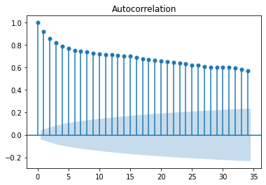
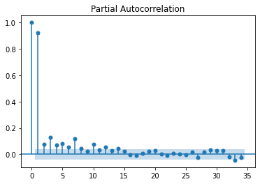
This indicates that the data is stationary. Another way to verify this is using the pdarima library to identify the lag at which the data will be stationary using adf, kpss and pp tests. While adf and pp are consistent with the above kpss test indicates that the data is stationary at d=1.
from pmdarima.arima.utils import ndiffs
## Adf Test
print(ndiffs(data.pm25, test='adf'))

# KPSS test
print(ndiffs(data.pm25, test='kpss'))

# PP test:
print(ndiffs(data.pm25, test='pp'))
0
1
0
Stepwise ARIMA
Performing stepwise arima in python to find the optimum p, d, q values.
import pmdarima as pm

# splitting into test and train
split_time = len(data)-365*2 # Latest two years is training, rest is test
time_train = data.date[:split_time]
x_train = data.pm25[:split_time]
time_valid = data.date[split_time:]
x_valid = data.pm25[split_time:]


model = pm.auto_arima(x_train, start_p=1, start_q=1,
                      test='adf',       # use adftest to find optimal 'd'
                      max_p=3, max_q=3, # maximum p and q
                      m=365,              # frequency of series
                      d=None,           # let model determine 'd'
                      seasonal=False,   # No Seasonality (as first trail)
                      start_P=0,
                      D=None,
                      trace=True,
                      error_action='ignore',
                      stepwise=True)
print(model.summary())
Performing stepwise search to minimize aic


 ARIMA(1,0,1)(0,0,0)[0]             : AIC=13312.056, Time=0.26 sec
 ARIMA(0,0,0)(0,0,0)[0]             : AIC=19910.319, Time=0.02 sec
 ARIMA(1,0,0)(0,0,0)[0]             : AIC=inf, Time=0.02 sec
 ARIMA(0,0,1)(0,0,0)[0]             : AIC=18004.728, Time=0.15 sec
 ARIMA(2,0,1)(0,0,0)[0]             : AIC=13203.466, Time=0.48 sec
 ARIMA(2,0,0)(0,0,0)[0]             : AIC=inf, Time=0.09 sec
 ARIMA(3,0,1)(0,0,0)[0]             : AIC=13204.966, Time=0.45 sec
 ARIMA(2,0,2)(0,0,0)[0]             : AIC=13204.925, Time=0.45 sec
 ARIMA(1,0,2)(0,0,0)[0]             : AIC=13249.558, Time=0.30 sec
 ARIMA(3,0,0)(0,0,0)[0]             : AIC=inf, Time=0.20 sec
 ARIMA(3,0,2)(0,0,0)[0]             : AIC=13207.206, Time=0.35 sec
 ARIMA(2,0,1)(0,0,0)[0] intercept   : AIC=13196.527, Time=1.07 sec
 ARIMA(1,0,1)(0,0,0)[0] intercept   : AIC=13270.440, Time=0.36 sec
 ARIMA(2,0,0)(0,0,0)[0] intercept   : AIC=13281.731, Time=0.17 sec
 ARIMA(3,0,1)(0,0,0)[0] intercept   : AIC=13197.878, Time=1.48 sec
 ARIMA(2,0,2)(0,0,0)[0] intercept   : AIC=13197.829, Time=1.33 sec
 ARIMA(1,0,0)(0,0,0)[0] intercept   : AIC=13305.106, Time=0.06 sec
 ARIMA(1,0,2)(0,0,0)[0] intercept   : AIC=13230.273, Time=0.55 sec
 ARIMA(3,0,0)(0,0,0)[0] intercept   : AIC=13252.937, Time=0.20 sec
 ARIMA(3,0,2)(0,0,0)[0] intercept   : AIC=13199.299, Time=1.87 sec

Best model:  ARIMA(2,0,1)(0,0,0)[0] intercept
Total fit time: 9.881 seconds
                               SARIMAX Results
==============================================================================
Dep. Variable:                      y   No. Observations:                 1584
Model:               SARIMAX(2, 0, 1)   Log Likelihood               -6593.264
Date:                Tue, 28 Dec 2021   AIC                          13196.527
Time:                        21:42:13   BIC                          13223.366
Sample:                             0   HQIC                         13206.498
                               - 1584
Covariance Type:                  opg
==============================================================================
                 coef    std err          z      P>|z|      [0.025      0.975]
------------------------------------------------------------------------------
intercept      0.5080      0.235      2.162      0.031       0.047       0.969
ar.L1          1.5900      0.030     53.575      0.000       1.532       1.648
ar.L2         -0.5941      0.029    -20.557      0.000      -0.651      -0.537
ma.L1         -0.8732      0.023    -38.503      0.000      -0.918      -0.829
sigma2       241.1973      4.922     49.000      0.000     231.550     250.845
===================================================================================
Ljung-Box (L1) (Q):                   0.17   Jarque-Bera (JB):              1164.77
Prob(Q):                              0.68   Prob(JB):                         0.00
Heteroskedasticity (H):               1.01   Skew:                             0.02
Prob(H) (two-sided):                  0.92   Kurtosis:                         7.20
===================================================================================
The error metrics for the test data is:
# Getting accuracy metrics on test data
results_model = model.predict(n_periods = 365*2)
results_model

from sklearn.metrics import mean_squared_error, mean_absolute_error
from math import sqrt
print('RMSE is ', sqrt(mean_squared_error(x_valid, results_model)))
print('MAE is ', mean_absolute_error(x_valid, results_model))
RMSE is  50.53383627717328
MAE is  43.4421801512105
From stepwise ARIMA, we see that the most optimal is p=2, d=0, and q=1 values with no significant seasonal component. This makes sense as any air pollutant generally stays in the air for a maximum of two days for Hyderabad wind and climatic patterns. So the effect of any sudden increase or decrease in pollutants (MA Component) exists for a day in the future. Also, the pollution today is effected by the baseline pollution in the last two days (AR component).
# Predicting on the complete data (test + train)
from statsmodels.tsa.arima_model import ARIMA
model_arima = ARIMA(data.pm25, order=(2,0,1))
results_AR = model_arima.fit(disp=-1)
plt.figure(figsize=(16,12), dpi= 80)
plt.plot(data.date, data.pm25)
plt.plot(data.date, results_AR.fittedvalues, color='red', alpha = 0.9)
plt.title("Actual vs predicted for PM 25 in Hyderabad", fontsize=20)
plt.show()
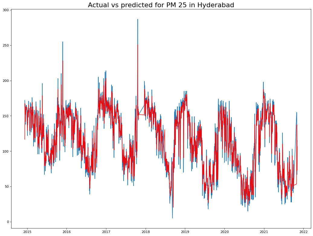
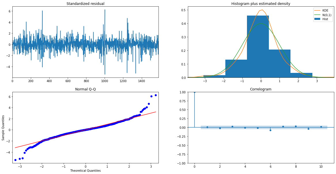
From the residuals we can see no patterns, indicating that we have a good prediction.
print(model.plot_diagnostics(figsize=(20,10)))
In the next blogs, we will implement deep learning (Like LSTM, RNN) and other methods on this data to deploy multiple models using various deployment methodologies.
References
- Class notes, Jiahua Wu, Logistics and Supply-Chain Analytics, MSc Business analytics, Imperial College London, Class 2020-22